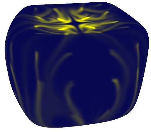
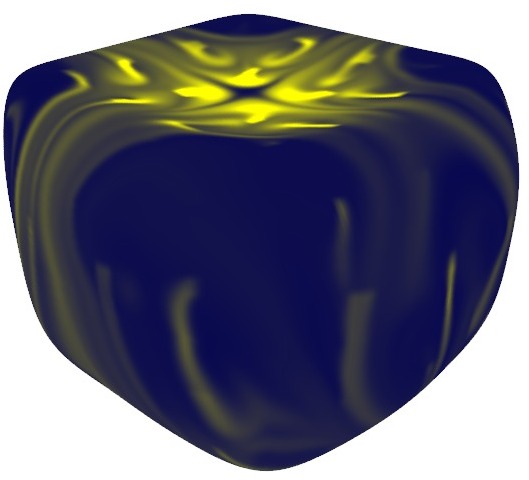
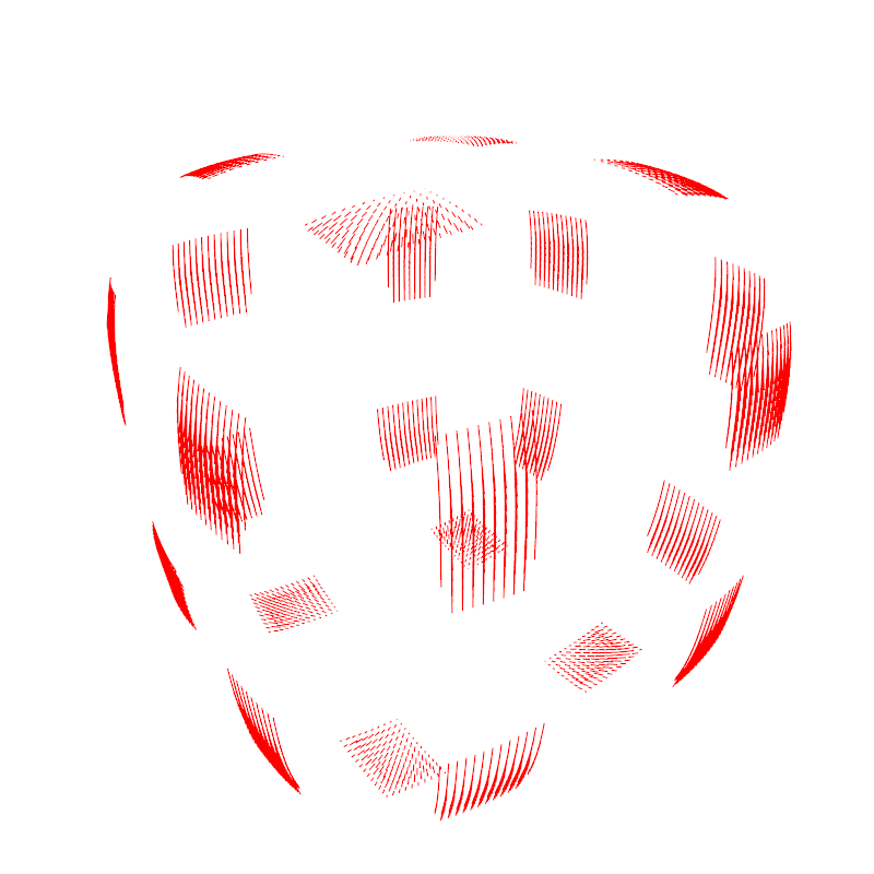
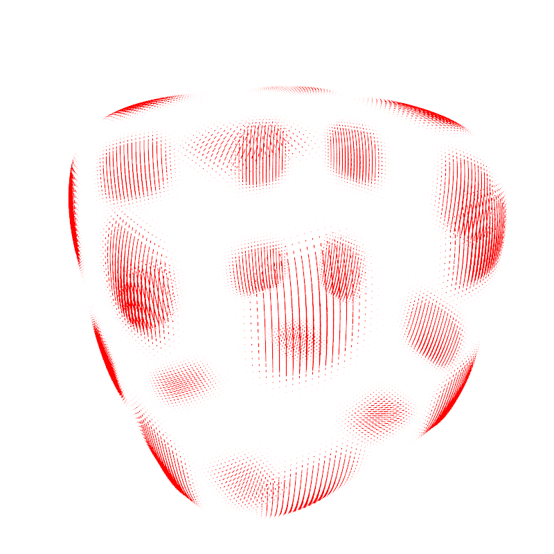
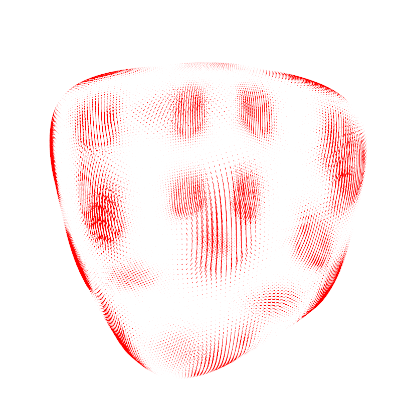
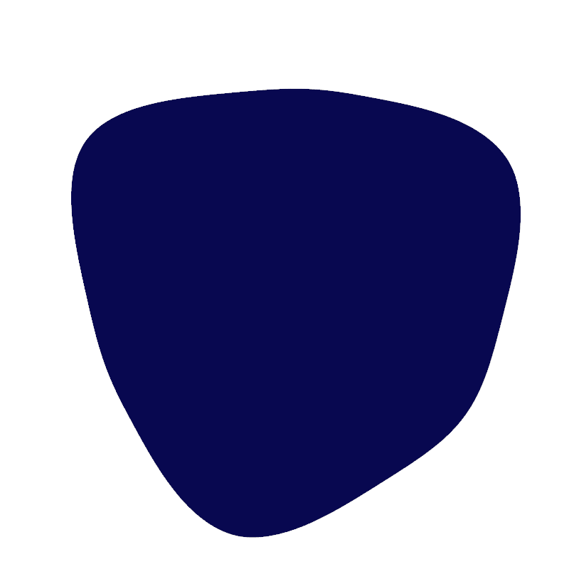
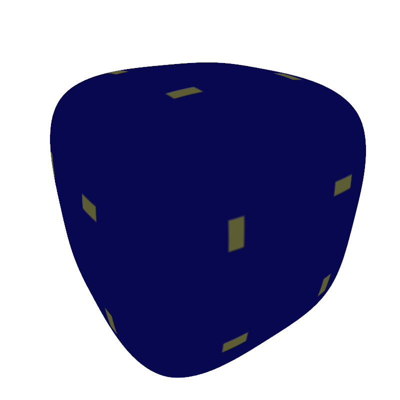
Example: Simulation of fluid on a closed surface.
In this work, we show how to calculate the Navier-Stokes equations on a smooth surface, where we want to simulate a fluid flow. We used a parametrization of a Catmull-Clark surface, from which we calculate a metric that depends on its tangent vectors and use this metric to get the necessary differential operators to solve the problem. The Navier-Stokes equations are solved on a discretization of the surface, dealing with the transition of the fluid between the patches that form the surface. This work is based in the work of Jos Stam.
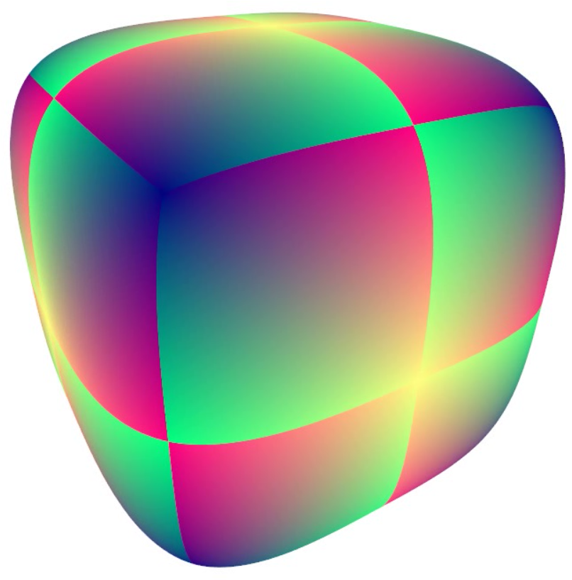
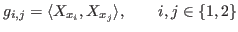
To simulate fluid we need to get a parametrization of some surface, one good candidate is a Catmull-Clark surface, which is smooth almost everywhere. Moreover, it is necessary to compare vectors in different points on the surface for fluid simulators, for example, velocity, force, etc.
The Navier-Stokes equations on a smooth surface are
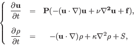
where


The equations are solved in four steps:
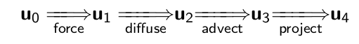
First, we solve this equation

which is discretized by
So we just sum the values of the external forces to the current velocity.
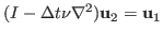
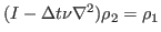
Now, we solve the diffusion equation

which is discretized by
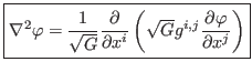
where the Laplacian operator is given by
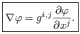
The advection equation is given by
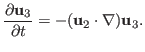
where the gradient operator is given by
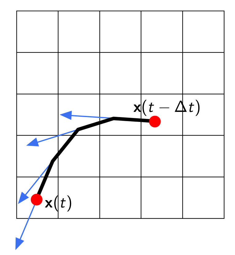
which is solved using a semi-Lagrangian technique, where we calculate the trajectory of each point of the grid to get its velocity in the previous time.
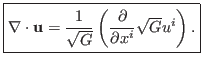
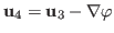
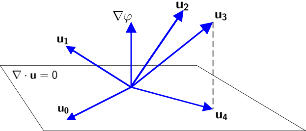
The result of the last step is projected

such that

where the divergent is given by
To find this projection we solve the Poisson equation

followed by
For the density field, we first solve this equation

which is discretized by
So we just sum the values from the sources to the current density.
Next, we solve the diffusion

which is discretized by
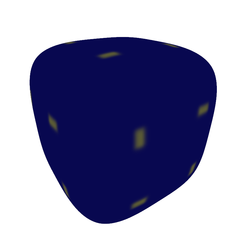
Finally, the advection equation is given by
which is solved also using a semi-Lagrangian technique.